
Neural Circuits: A new generalized framework for training arbitrarily connected recurrent networks with multiplicative gating
Recurrent Neural Networks (RNN) have seen both hype and disappointment in the past several decades. In theory, they can represent spatiotemporal relationships of infinite complexity, and pick out causal patterns the occur through time. In practice, most RNN have disappointed. However, research into Long Short Term Memory (LSTM) has given hope to the potential of recurrent networks. Neural Circuits are my approach to building and training recurrent networks, heavily inspired by LSTM and a more general variant: LSTM-g.
RNN Quick History
A simple version of a RNN adds a self-recurrent connection to the hidden layer of a feed-forward ANN. This allows the hidden layer to update its internal state using both the current input and the previous state. Theoretically, a large-enough RNN can approximate any temporal function. Sadly, though, there is a nagging problem of limited representation horizon due to vanishing and/or exploding gradients; creating instability or ineffectiveness in the training algorithm. As the time between signal and response gets longer, there is more and more noise destroying the power of that signal. Many thought recurrent networks were not worth the trouble, and moved on to more successful (and simpler) techniques.
In the late 1990’s, Sepp Hochreiter and Jurgen Schmidhuber published a paper called “Long Short-Term Memory”, and the field changed. All of a sudden, there was a technique to apply neural networks to noisy time-series problems with long lags between cause and effect.
In LSTM, a special layer holds onto memory indefinitely (until instructed to forget). This memory cell has a self-recurrent connection with a constant weight of 1, allowing it to pass error through it’s backpropagation step unaltered. Due to this property, the memory cell was termed a constant error carousel (CEC).
A LSTM block is composed of an input layer, output layer, memory cell, and three special gating layers:
- Input gate: filters input into the memory cell;
- Forget gate: controls when the memory cell should remember/forget its last state;
- Output gate: filters the output of the memory cell.
Together these three gating layers can accumulate and store data for arbitrarily long periods of time, vastly outperforming vanilla RNNs in almost all medium to long term temporal modeling. Over the past 20 years, LSTMs have been applied to music composition, language processing, phoneme recognition, and many other problems which depend on time.
In 2012, Derek Monner published a new perspective to the LSTM paradigm, termed Generalized LSTM (LSTM-g). In this, he reinterpreted LSTM gating to act on connections (as opposed to acting directly on the layer activations). By avoiding truncated error propagation, he allowed for more flexible architectures. In addition, he was able to maintain learning rules that are local in space and time (and thus much more biologically plausible). Most researchers now train using the computationally expensive algorithm Backpropagation Through Time (BPTT), presumably under the assumption that computational power is cheap. I’d agree with them if I also worked at Google…
Why create another neural network framework?
When it comes to convolutional neural nets, trained through classic backpropagation, there are many viable options (TensorFlow, Theano, Torch…). Most frameworks provide efficient code which can offload much of the work onto the GPU. However RNNs are typically a sore spot. The easy automated solution for learning recurrent networks is a technique called Truncated BackPropagation Through Time (TBPTT). The technique amounts to storing a complete history of the state and calculations for the last T timesteps, and backpropagating errors through the network unrolled through time (see this or this for a good visual of an unrolled network, as well as more background on recurrent networks).
Learning from stored history is a problem for large networks, or those with many recurrent connections, or those with long-range temporal dynamics (i.e. when events far in the past have significant impact). Put another way, it is a problem for every real-world model. Practitioners are faced with deciding between:
- a good model,
- a slow model, or
- a resource-intensive model.
Time is money, so the current trend is for resource-intensive training.
An analogy comparing your typical TBPTT algorithm vs an online variant: Joe and Sue are running a marathon (26.2 miles), with city landmarks every mile. However, every time Joe passes a new landmark, he is magically teleported back to the starting line, and 10 pounds is added to his (large) backpack. To advance $T$ miles, he must actually run $M$ miles, and by that time he will have accumulated $W$ additional pounds of weight, where:
\[M = \sum_{i=1}^T{I} \\ W = 10T\]By the end of the marathon, Joe has traveled 377.2 miles and completed the final 26.2 miles with an additional 260 pounds of weight. I’ll let you decide who is likely to win (though it’s impressive that Joe can finish the race at all!)
I wanted to build a framework that, from the ground up, could be good, fast, and lightweight (all at the same time).
Introduction to Neural Circuits
The concept is simple. Neural network layers (hereafter called nodes) no longer connect to each other directly, they connect through intermediate gates. A gate $g$ is a multiplicative integrator, receiving input from one or more nodes and applying a learned weight matrix $w_g$. The set of nodes projecting input data to gate $g$ is $I_g$, and the node to which the gate projects is $O_g$.
The gate’s state is:
\(\begin{align} s_g(τ) = w_g(τ) \prod_{i ∈ I_g} {\hat y}_i(τ) \end{align}\) where: \(\begin{align} {\hat y}_i(τ) = \begin{cases} y_i(τ), & \text{if node } O_g \text{ comes after node } i \\ y_i(τ-1), & \text{otherwise} \end{cases} \end{align}\)
As hinted at in equation (2), there is an explicit ordering to the nodes, where the input unit is the first, and the output unit is the last. On presentation of a new input, nodes are activated in order, and store key values for the learning step.
Every gate projects to exactly one node, however nodes can receive projections from any number of gates. After summing gate inputs $s_g$, the node then adds a bias term $b_j$ and applies an activation function $f_j$ (sigmoid, ReLU, or any other everywhere-differentiable function). For a node $j$, the output $y_j$ is:
\[\begin{align} s_j(τ) = \sum_{g ∈ I_j}{s_g(τ)} + b_j(τ) \end{align}\] \[\begin{align} y_j(τ) = f_j(s_j(τ)) \end{align}\]That’s it. The rest is up to the network designer.
Building a Network
To get you comfortable with this simplistic network concept, lets walk through a few examples. We’ll be using MIT-licensed packages that I’ve designed and developed for the Julia programming language: Plots and OnlineAI. After installing and starting Julia, you can install these packages:
# install Plots and checkout the latest version
Pkg.add("Plots")
Pkg.checkout("Plots")

# install OnlineAI
Pkg.clone("https://github.com/tbreloff/OnlineAI.jl")

# we'll be using the Gadfly backend for these examples
Pkg.add("Gadfly")
Then you can load and initialize:
using OnlineAI, Plots
gadfly()
Lets build a simple recurrent network with multiplicative nodes:
# create the nodes
input = Node(3, tag = :input)
hidden1 = Node(3, SigmoidActivation(), tag = :hidden1)
hidden2 = Node(3, SigmoidActivation(), tag = :hidden2)
output = Node(1, tag = :output)

# define our circuit (node order matters)
rnn = Circuit([input, hidden1, hidden2, output])

# create the gates (connections)
project!([hidden1], hidden1, tag = :hh1)
project!([input, hidden2], hidden1, tag = :ih1)
project!([input, hidden1, hidden2], hidden2, tag = :h2)
project!([input, hidden1, hidden2], output, tag = :o)
And then visualize the network with Plots:
plot(rnn, node_x = [0.5,0.3,0.7,0.5])
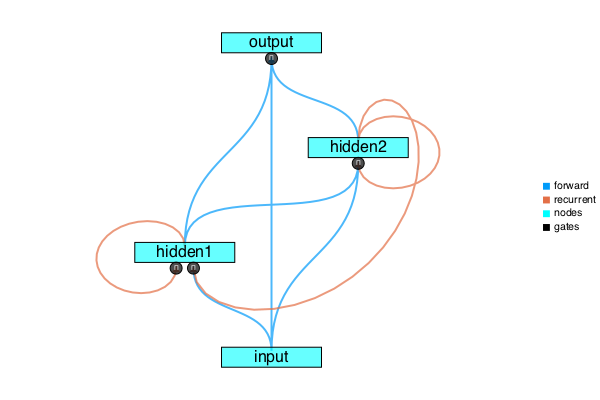
Figure A: Directed Graph for our RNN
The small black circles represent the multiplicative gates. The gate outputs are then summed by the corresponding node, and an activation function is applied. The color of the curve corresponds to the conditional in the equation of ${\hat y}_i(τ)$ above.
That example was quick, but in Julia we can make things uber-simple. Here’s the same network, built with serious convenience:
rnn = circuit"""
3 input             # Comments are allowed.
3 hidden1 sigmoid   # First argument is the number of cells.
3 hidden2 sigmoid   # Remaining arguments are activation type and tag.
1 output            #   (they can come in any order)
"""

gates"""
rnn                           # First line should be the circuit.
hidden1 --> hidden1 ; hh1     # Separate mapping from arguments with a semicolon.
1,3     --> 2       ; ih1     # Can use the node indices instead of tags.
1,2,3   --> hidden2 ; h2      # Arguments are comma separated, and can define
1,2,3   --> output  ; ALL, o  #   the connection type, and assign a tag.
"""
LSTM
Here’s an LSTM network, wrapped in a function call (we’ll re-use this later):
function create_lstm(nin::Integer, nout::Integer; tag=gensym("lstm"))
    lstm = circuit"""
        nin  input
        nin  inputgate  sigmoid
        nin  forgetgate sigmoid
        nin  memorycell
        nin  outputgate sigmoid
        nout output
    """
    lstm.tag = tag

    gates""" lstm
        1   --> 2,3,5,6
        3,4 --> 4 ; FIXED  # CEC
        1,2 --> 4          # gated input
        4,5 --> 6          # gated output
        4   --> 2,3,5      # peepholes
    """
end
Learning
Neural Circuits use a gradient-based online backpropagation algorithm, similar to Real Time Recurrent Learning (RTRL). Given an error function $E(\tau)$, our goal will be to minimize a discounted sum of errors (our cost):
\[\begin{align} C(τ) &= \sum_{i=0}^∞{γ^i E(τ-i)} \\ &= γ C(τ-1) + E(τ) \end{align}\]LSTM gates are a specific version of the perspective above. Given two nodes projecting to the same gate, if one has a sigmoid activation it can act as an LSTM gate. Of course, one might find alternate activations to give richer behavior, such as a $tanh$, which could “gate and negate” a paired input.
Notes
A gate is the generalization of Derek Monner’s algorithm LSTM-g, which is in turn a generalization of LSTM.