A couple of months ago, I noticed a drop off in my output. It came as a surprise and I started to wonder if the bike had become miscalibrated over time. I discovered that you can download your workout history from the Peloton site and decided it was time to dig into the numbers. Did my workout output, frequency, or content change to justify a 10% drop in ability?
I downloaded my data and put together a Jupyter notebook to visualize my progress. After a bit of exploring, I made a bare-bones repo and pushed it up to github: pelonalysis.
My discovery? I was working twice as much during my initial months!
Sadly I can no longer blame my bike. Time to get to work!
]]>As I’m a fan of metaphors, I’ll liken the goal of general AI to the goal of inventing a car.
Decades ago, researchers had a big effort in knowledge engineering and logical reasoning. The path towards human-level AI seemed obvious; we must encode enough world knowledge into a system, and give it the correct algorithms to draw on that world knowledge.
In my metaphor, they were designing steering wheels, speedometers, and other devices that were intended for human understanding and communication while driving.
We made great progress, but that work was largely unusable for practical applications. I mean seriously… who wants a steering wheel without anything to drive?! Many critics concluded that the efforts were wasted, and that the approaches were fundamentally flawed.
Also decades ago, we saw the invention of the core mathematics and inventions driving advances in neural networks. Backpropagation, feed-forward neural nets, convolutional layers, and Long-Short-Term-Memory (LSTM) are examples of things that existed a long time ago, but have only hit their stride in the last few years.
In my metaphor, we developed the wheels and chassis, along with the required physics understanding of torque and friction.
However, despite high expectations, this also disappointed initially, since what good is a cart without a horse to pull it? This disappointment led to an AI winter, until…
In the early part of this decade, a group of researchers discovered that with enough compute power, old techniques using neural networks could perform very well in sensory-motor domains such as image recognition and speech-to-text. They had found a horse to pull their dusty old cart!
Rather, they now had an engine! Combining the “engine” with the “wheels” allowed for numerous applications, with seemingly limitless possibilities. However, all that power is limited to very narrow domains: asking Echo to play a song, or getting calendar entries from Siri, or making a haircut appointment with Duplex.
Without the ability to interface seamlessly with humans, the technology must stay “on the rails”, like a train.
Now, no one can deny that railways were both useful and transformative. They paced the way for efficient trade and globalization of economies. But while railways were important for industry, they had less impact on the day to day lives of people. It was, quite simply, not as transformative as the automobile.
We’ve separately invented the steering wheel and controls (world knowledge and logical reasoning), the tires and the chassis (statistical models aka Deep Learning), and a powerful engine (CPUs, GPUs, and TPUs… oy my!). But we don’t have a car (AI).
I think Gary, Judea, and others simply feel this: no one has invented the car, and we won’t get there by improving the tires. We shouldn’t choose between logic or statistics… we should build a system that uses both! It works for humans, after all.
]]>Instead, the world will be run by neural networks. Why not? They’re really great at recognizing objects in images, winning at board games, and even writing movie scripts. (Well maybe not movie scripts.)
I can’t decide if he’s being naive or if we should be scared (no… not from an army of infinitely intelligent super-robots).
Neural networks are very powerful. There’s no question. But human software engineers do more than just pattern match inputs into outputs. In software development, it’s not enough to produce correct outputs 99% of the time (though even that is seemingly unachievable for most complex tasks). Imagine if your bank deposits only landed in the right account 99% of the time. Or if an air traffic control tower only assured your plane would land safely 99% of the time.
There are too many tasks that require near-certain guarantees on performance. And most importantly, many of those tasks require full human understanding of the processes and algorithms which determine the outcome. This is something we simply cannot expect from end-to-end neural (statistical) models.
I think he’s naive for claiming that statistical modeling can replace good ol’ fashion software engineering.
Neural networks are fragile, complicated, opaque, compute-heavy, and easily tricked. They are simultaneously hard to understand and easy for bad actors to manipulate. But… they get some amazing results in certain domains (most notably sensorial tasks like vision, hearing, and speech).
Humans are gullible animals. We have implicit biases, and constantly change the facts to match our understanding of the world. In a world filled with Software 2.0, where the software programs are written by statistical models, the output of that software will start to look like magic. So much so that people will start to believe that it is magic.
Throughout history, people have been happy to worship and serve a power greater than them. What if people start to believe in computing magic, and trust important life decisions to a statistical model? Insurance companies might deny your coverage because a neural network told them a procedure wouldn’t help you. Employers will discriminate based on expected performance. Police will monitor and arrest people through statistical profiling, predicting crime that hasn’t yet happened. Courts will prosecute and sentence based on expectations of repeat offense.
You might be saying… “This is already happening!” I know. I think we should be scared of relying on statistical models without properly accounting for their biases and shortcomings.
Just like the spreading IoT time bomb, placing blind trust in Software 2.0 is a trojan horse. We let it into our lives without full understanding, and it puts us at risk in ways we can’t realize.
The path forward is in developing human-led technology. Building machines that can help and advise, but do not assert full control. We shouldn’t worship a machine, and we shouldn’t put our blind trust in statistical methods. Humans are more than just pattern matchers. We can transfer our experience to new environments. We can plan and reason, without having to fail at a task millions of times first.
Instead of rushing to Software 2.0, lets view neural networks in proper context: they are models, not magic.
]]>In this post I wanted to provide some perspective on the Plots project, from origin to today, as well as to speculate on its future. If you have further questions about this project (or any of my other open source efforts), please use the public forums (Github, Discourse, Gitter, Slack) to seek help from other users and developers, as I have very little capacity to answer emails or messages sent directly to me. (Not to mention I probably won’t have the most up to date answer!)
I spent my career in finance building custom visualization software to analyze and monitor my trading and portfolios. When I started using Julia, the visualization options were not exciting. Most available packages were slow, lacking features, or cumbersome to use (or all of those things). As both the primary designer and user of my software in my previous roles, I knew a better approach was possible.
In 2015, early in my Julia experience, I created Qwt.jl, a Julia interface to a slightly customized wrapper of the Qwt visualization framework. I used it primarily to analyze trading simulations and watch networks of spiking neurons fire. It was (IMO) a massive step up in cleanliness and usability compared to my experiences doing visualization in Python, C++, and Java. I am a nut for convenience, and made sure all the defaults were set such that 90% of the time they were exactly what I wanted. Qwt.jl could be thought of as the design inspiration for the API of Plots.
In August of 2015, a bunch of devs in the Julia community (most of which had “competing” visualization packages) set up the JuliaPlot (note the missing “s”) organization to discuss the state of Julia visualization. We all agreed that the community was too fragmented but most thought it was too hard a problem to tackle properly. Each package had many strengths and weaknesses, and there was large difference in supported feature sets and API style.
I laid out a rough plan for “one interface to rule them all”. It was not well received, with the biggest objection that it wasn’t likely to be successful. People, after all, have very different preferences in naming, styles, and requirements. It would be impossible to please enough people enough of the time to make the time investment worthwhile. Now, telling me something is impossible is an effective way to motivate me. I pushed the initial commits of Plots that weekend.
Plots (and the larger JuliaPlots ecosystem) has been (again, IMO) a wildly successful project. Is it perfect? Of course not. Nothing is. There are precompilation issues, unsatisfying customization of legends, minimal interactivity, and more. But it has received a large following of loyal users and (much more important) dedicated contributors and maintainers.
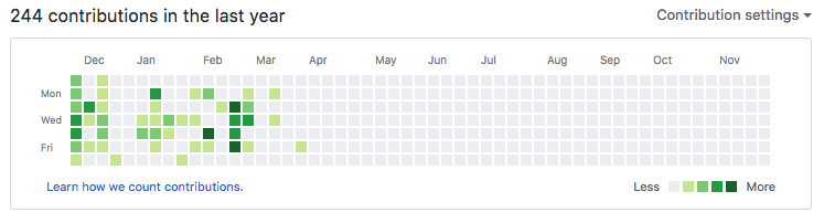
Sadly, I don’t have the ability to work on the project, as described above. In fact, I bet you can guess when I joined Elemental Cognition given my Github activity:
However, even though I’ve backed away from the project, it is in good hands with many people invested in its continued success. Looking at the list of contributors to Plots (64 people at the time of writing this post) and the graph of commits (below), it seems very clear that this is an active and passionate community of Julia visualizers that care about the success of the ecosystem.
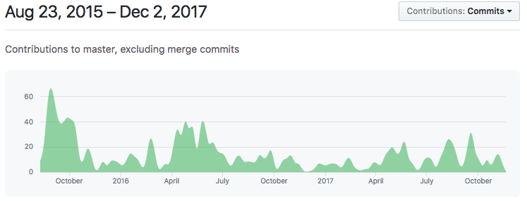
In fact, this graph seems to show that activity has risen since I handed over responsibility of the organization to the JuliaPlots team. I reason that my departure gave other members the courage to take a more active role, before which their contributions were not as aggressive and passionate.
The design of RecipesBase and the recipes concept has ensured that, even if something better comes along to replace the Plots core, things like StatPlots, PlotRecipes, and many other custom recipes can still be used. This is a motivating idea when deciding whether to invest time in a project… knowing that a contributed recipe can outlast the plotting package it was designed for. This is a primary reason that I expect JuliaPlots to remain active and vibrant.
There are many ways to make visualization in Julia better. We need better compilation performance, fewer bugs, better support for interactive workflows, more complete documentation, as well as countless other issues. The number of things that can be improved is a testament to how insanely difficult it is to build a visualization platform. It’s perfectly natural to have 10 different solutions, because there are 1,000 different ways to look at a dataset. How could one solution possibly cover everything?
During (and after) JuliaCon 2016, Simon Danisch and I had a bunch of brainstorming sessions diving into how we could improve the core Plots engine. These conversations were mostly centered around strategies to support better performance and interactivity in the Plots API and core loop. We also wanted to give backends more control over lazily recomputing attributes and data, and optional updates to subparts of the visualization (when few things have changed). The goal was marrying extreme flexibility with extreme performance (similar to the goal of Julia itself).
I hope that Simon’s latest project MakiE is the realization of those ideas and goals. I would consider it a big success if he could replace the core of Plots with a new engine, without losing any of the flexibility and features that currently exist. Of course, it will be a ridiculously massive effort to achieve feature-parity without tapping into recipes framework and the Plots API. So my skepticism rests on the question of whether the existing concepts can be mapped into a MakiE engine. I wish Simon the best of luck!
Aside from large rebuilds, there is some low-hanging fruit to a better ecosystem, some of which will be helped by things like “Pkg3” and other core Julia improvements. Also, the (eventual) release of Julia 1.0 will bring a wave of new development effort to fill in the gaps and add missing features.
All things told, I have high hopes for the future of Julia and especially the visualization, data science, and machine learning sub-communities within. I hope to find my way back to the language someday!
]]>In recent research from Arild Nøkland, he explores extensions to random feedback (see part one) that avoid backpropagating error signals sequentially through the network. Instead, he proposes Direct Feedback Alignment (DFA) and Indirect Feedback Alignment (IFA) which connect the final error layer directly to earlier hidden layers through random feedback connections. Not only are they more convenient for error distribution, but they are more biologically plausible as there is no need for weight symmetry or feedback paths that match forward connectivity. A quick tutorial on the method:
In this post, we’re curious whether we can use a surrogate gradient algorithm that will handle threshold activations. Nøkland connects the direct feedback connections from the transformation output error gradient to the “layer output”, which in this case is the output of the activation functions. However, we want to use activation functions with zero derivative, so even with direct feedback the gradients would be zeroed during propagation through the activations.
To get around this issue, we modify DFA to instead connect the error layer directly to the inputs of the activations, instead of the outputs. The result is that we have affine transformations which can learn to connect latent input ($h_{i-1}$ from earlier layers) to a projection of output error ($B_i \nabla y$) into the space of $h_i$, before applying the threshold nonlinearity. The effect of the application of a nonlinear activation is “handled” by the progressive re-learning of later network layers. Effectively, each layer learns how to align their inputs with a fixed projection of the error. The hope is that, by aligning layer input with final error gradients, we can project the inputs to a space that is useful for later layers. Learning happens in parallel, and later layers eventually learn to adjust to the learning that happens in the earlier layers.
Reusing the approach in an earlier post on JuliaML, we will attempt to learn neural network parameters both with backpropagation and our modified DFA method. The combination of Plots and JuliaML makes digging into network internals and building custom learning algorithms super-simple, and the DFA learning algorithm was fairly quick to implement. The full notebook can be found here. To ease understanding, I’ve created a video to review the notebook, method, and preliminary results:
Nice animations can be built using the super-convenient animation facilities of Plots:
The concept of Target Propagation (targetprop) goes back to LeCun 1987, but has recently been explored in depth in Bengio 2014, Lee et al 2014, and Bengio et al 2015. The intuition is simple: instead of focusing solely on the “forward-direction” model ($y = f(x)$), we also try to fit the “backward-direction” model ($x = g(y)$). $f$ and $g$ form an auto-encoding relationship; $f$ is the encoder, creating a latent representation and predicted outputs given inputs $x$, and $g$ is the decoder, generating input representations/samples from latent/output variables.
Bengio 2014 iteratively adjusts weights to push latent outputs $h_i$ towards the targets. The final layer adjusts towards useful final targets using the output gradients as a guide:
\[\begin{align} \hat{h}_i &= g_i (\hat{h}_{i+1}) \nonumber \\ \Delta \hat{h}_M &= -\eta \frac{\partial L}{\partial y_M} \nonumber \end{align}\]Difference Target Propagation makes a slight adjustment to the update, and attempts to learn auto-encoders which fulfill:
\[\begin{align} \hat{h}_i - h_i &= g_i (\hat{h}_{i+1}) - g_i (h_{i+1}) \nonumber \end{align}\]Finally, Bengio et al 2015 extend targetprop to a Bayesian/generative setting, in which they attempt to reduce divergence between generating distributions p and q, such that the pair of conditionals form a denoising auto-encoder:
\[\begin{align} h_i &\sim p (h_i | \hat{h}_{i+1}) \nonumber \\ h_i &\sim q (h_i | \hat{h}_{i-1}) \nonumber \end{align}\]Targetprop (and its variants/extensions) is a nice alternative to backpropagation. There is still sequential forwards and backwards passes through the layers, however we:
Equilibrium Propagation (e-prop) is a relatively new approach which (I’m not shy to admit) I’m still trying to get my head around. As I understand, it uses an iterative process of perturbing components towards improved values and allowing the network dynamics to settle into a new equilibrium. The proposed algorithm alternates between phases of “learning” in a forward and backward direction, though it is a departure from the simplicity of backprop and optimization.
The concepts are elegant, and it offers many potential advantages for efficient learning of very complex networks. However it will be a long time before those efficiencies are realized, given the trend towards massively parallel GPU computations. I’ll follow this line of research with great interest, but I don’t expect it to be used in a production setting in the near future.
A recent paper from DeepMind takes an interesting approach. What if we use complex models to estimate useful surrogate gradients for our layers? Their focus is primarily from the perspective of “unlocking” (i.e. parallelizing) the forward, backward, and update steps of a typical backpropagation algorithm. However they also offer the possibility of estimating (un-truncated) Backpropagation Through Time (BPTT) gradients, which would be a big win.
Layers output to a local model, called a Decoupled Neural Interface. This local model estimates the value of the backpropagated gradient that would be used for updating the parameters of that layer, estimated using only the layer outputs and target vectors. If you’re like me, you noticed the similarity to DFA in modeling the relationship of the local layer and final targets in order to choose a search direction which is useful for improving the final network output.
I think the path forward will be combinations and extensions of the ideas presented here. Like synthetic gradients and direct feedback, I think we should be attempting to find reliable alternatives to backpropagation which are:
Obviously they must still enable learning, and efficient/simple solutions are preferred. I like the concept of synthetic gradients, but wonder if they are optimizing the wrong objective. I like direct feedback, but wonder if there are alternate ways to initialize or update the projection matrices ($B_1, B_2, …$). Combining the concepts, can we add non-linearities to the error projections (direct feedback) and learn a more complex (and hopefully more useful) layer?
There is a lot to explore, and I think we’re just at the beginning. I, for one, am happy that I chose the red pill.
]]>Backpropagation is fairly straightforward, making use of some basic calculus (partial derivatives and the chain rule), and matrix algebra. Its goal: to measure the effect of internal parameters of a model on the final loss (or cost) of our objective. This value is called the gradient of our parameters with respect to the loss. For input x, target y, model f, and model parameters $\theta$:
\[\nabla_\theta = \frac{\partial L(f(x,\theta), y)}{\partial \theta} = \frac{\partial L}{\partial \theta} = \frac{\partial L}{\partial f} \frac{\partial f}{\partial \theta}\]For a quick review of the backpropagation method, see this short video:
For a commonly used linear transformation:
\[\begin{align} y &= w x + b \nonumber \\ \theta &= \{w, b\} \nonumber \end{align}\]we typically multiply the backpropagated gradient by the transpose of the weight matrix: $w^T$. This is the mathematically correct approach to computing the exact gradient:
\[\begin{align} \nabla_w &= \nabla_y x^T \nonumber \\ \nabla_b &= \nabla_y \nonumber \\ \nabla_x &= w^T \nabla_y \nonumber \end{align}\]All was right with the world, until I read Random feedback weights support learning in deep neural networks. In it, Lillicrap et al describe how you can replace $w^T$ with a random and fixed matrix $B$ during the backward pass so that:
\[\nabla_x = B \nabla_y\]And the network will still learn. WTF?! How could you possibly learn something from random feedback? It was as if I was no longer Mr. Anderson, but instead some dude sitting in goo with tubes coming out of my body. Why did I just choose the red pill?
To gain intuition about how random feedback can still support learning, I had to step back and consider the function of neural nets. First there are many exactly equivalent formulations of a neural net. Just reorder the nodes of the hidden layers (and the corresponding rows of the weight matrix and bias vector and the columns of downstream weights), and you’ll get the exact same output. If you also allow small offsetting perturbations in the weights and biases, the final output will be relatively close (in the non-rigorous sense). There are countless ways to alter the parameters in order to produce effectively equivalent models.
Intuitively we may think that we are optimizing a function like:
But in reality, we are optimizing a function like:
Vanilla backpropagation optimizes towards the surface valley (local minimum) closest to the initial random weights. Random feedback first randomly picks a valley and instead optimizes towards that. In the words of Lillicrap et al:
The network learns how to learn – it gradually discovers how to use B, which then allows effective modification of the hidden units. At first, the updates to the hidden layer are not helpful, but they quickly improve by an implicit feedback process that alters W so that $e^T W B e > 0$.
We implicitly learn how to make W approximately symmetric with B before searching for the local minimum. Wow.
Trying to intuit random feedback felt similar to my process of understanding Dropout. In a nutshell, Dropout simulates an ensemble model of $2^n$ sub-models, each composed of a subset of the nodes of the original network. It avoids overfitting by spreading the responsibility. Except it’s not a real ensemble (where models are typically learned independently), but instead some sort of co-learned ensemble. The net effect is a less powerful, but usually more general, network. The explanation I see for why Dropout is beneficial is frequently: “it prevents co-adaption of latent features”. Put another way, it prevents a network from acquiring weights that force a dependence between latent (hidden) features.
In backpropagation, the gradients of early layers can vanish or explode unless the weights and gradients of later layers are highly controlled. In a sense, we see co-adaption of weights across layers. The weights of earlier layers are highly dependent on the weights of later layers (and vice-versa). Dropout reduces co-adaption from intra-layer neurons, and random feedback may help reduce co-adaption from inter-layer weights.
Some will claim that random feedback is more biologically-plausible, and this is true. However the real benefit comes from breaking the fragile dependence of early-layer weight updates from later-layer weights. The construction of the fixed feedback matrices ${B_1, B_2, …, B_M}$ can be managed as additional hyperparameters and have the potential to stabilize the learning process.
Random feedback is just the tip of the iceberg when it comes to backprop-free learning methods (though random feedback is more a slight modification of backprop). In part 2, I’ll review more research directions that have been explored, and highlight some particularly interesting recent methods which I intend on extending and incorporating into the JuliaML ecosystem.
]]>If you have questions or want to request video tutorials on other topics, come chat.
]]>For questions, comments, or if you’re interested in collaborating, please join the JuliaML Gitter chat.
]]>Training deep neural networks (and likewise recurrent networks which are deep through time) with gradient descent has been a difficult problem, partially (mostly) due to the issue of vanishing and exploding gradients. One solution is to normalize layer activations, and learn the skew (b) and scale (g) as part of the learning algorithm. Online layer normalization can be summed up as learning parameter arrays g and b in the learnable transformation:
\[\begin{align} y &= g \odot z + b \\ where: z_o &= \frac{a_o - \mu_t}{\sigma_t} \\ a_o &= \sum_i{w_{oi} x_i} \\ \mu_t &= \alpha_t (\frac{1}{D} \sum_p{a_p}) + (1-\alpha_t) \mu_{t-1} \\ \sigma_t &= \alpha_t \sqrt{\frac{1}{D-1} \sum_p{(a_o - \mu_t)^2}} + (1-\alpha_t) \sigma_{t-1} \end{align}\]The vector a is the input to our LayerNorm layer and the result of a Linear transformation of x. We keep a running mean ($\mu_t$) and standard deviation ($\sigma_t$) of a using a time-varying weighting factor ($\alpha_t$).
Due mostly to LaTeX-laziness, I present the derivation in scanned form. A PDF version can be found here.
Layer normalization is a nice alternative to batch or weight normalization. With this derivation, we can include it as a standalone learnable transformation as part of a larger network. In fact, this is already accessible using the nnet
convenience constructor in Transformations:
using Transformations
nin, nout = 3, 5
nhidden = [4,5,4]
t = nnet(nin, nout, nhidden, :relu, :logistic, layernorm = true)
Network:
Chain{Float64}(
Linear{3-->4}
LayerNorm{n=4, mu=0.0, sigma=1.0}
relu{4}
Linear{4-->5}
LayerNorm{n=5, mu=0.0, sigma=1.0}
relu{5}
Linear{5-->4}
LayerNorm{n=4, mu=0.0, sigma=1.0}
relu{4}
Linear{4-->5}
LayerNorm{n=5, mu=0.0, sigma=1.0}
logistic{5}
)
A computation graph, or data flow graph, is a representation of math equations using a directed graph of nodes and edges. Here’s a simple example using Mike Innes’ cool package DataFlow. I’ve built a recipe for converting DataFlow graphs to PlotRecipes graphplot calls. See the full notebook for complete Julia code.
We’ll compute $f(x) = w * x + b$:
g = @flow f(x) = w * x + b
plot(g)
The computation graph is a graphical representation of the flow of mathematical calculations to compute a function. Follow the arrows, and do the operations on the inputs. First we multiply w and x together, then we add the result with b. The result of the addition is our output of the function f.
When x/w/b are numbers, this computation flow is perfectly easy to follow. But when they are tensors, the graph is much more complicated. Here’s the same example for a 1D, 2-element version where w is a 2x2 weight matrix and x and b are 2x1 column vectors:
plot(@flow f(x) = out(w11*x1 + w12*x2 + b1, w21*x1 + w22*x2 + b2))
Already this computational graph is getting out of hand. A tensor computation graph simply re-imagines the vector/matrix computations as the core units, so that the first representation ($f(x) = w * x + b$) is used to represent the tensor math which does a matrix-vector multiply and a vector add.
Making the jump from computation graph to tensor computation graph was a big improvement in complexity and understanding of the underlying operations. This improvement is the core of frameworks like TensorFlow. But we can do better. In the same way a matrix-vector product
\[(W*x)_i = \sum_j W_{ij} x_j\]can be represented as simply the vector $Wx$, we can treat the tensor transformation $f(x) = wx + b$ as a black box function which takes input vector (x) and produces output vector (f(x)). Parameter nodes (w/b) are considered learnable parameters which are internal to the learnable transformation. The new transformation graph looks like:
plot(@flow f(x) = affine(x))
Quite the improvement! We have created a modular, black-box representation of our affine transformation, which takes a vector input, multiplies by weight vector and adds a bias vector, producing a vector output:
And here’s the comparison for a basic recurrent network:
g = @flow function net(x)
hidden = relu( Wxh*x + Whh*hidden + bh )
y = logistic( Why*hidden + Wxy*x + by )
end
The unfortunate climate of ML/AI research is: “TensorFlow is love, TensorFlow is life”. If it can’t be built into a TF graph, it’s not worth researching. I think we’re in a bit of a deep learning hype bubble at the moment. Lots of time and money is poured into hand-designed networks with (sometimes arbitrary) researcher-chosen hyperparameters and algorithms. Your average high school student can install and build a neural network to perform quite complex and impressive models. But this is not the path to human-level intelligence. You could represent the human brain by a fully connected deep recurrent neural network with a billion neurons and a quintillion connections, but I don’t think NVIDIA has built that GPU yet.
I believe that researchers need a more flexible framework to build, test, and train complex approaches. I want to make it easy to explore spiking neural nets, dynamically changing structure, evolutionary algorithms, and anything else that may get us closer to human intelligence (and beyond). See my first post on efficiency for a little more background on my perspective. JuliaML is my playground for exploring the future of AI research. TensorFlow and competitors are solutions to a very specific problem: gradient-based training of static tensor graphs. We need to break the cycle that research should only focus on solutions that fit (or can be hacked into) this paradigm. Transformations (the Julia package) is a generalization of tensor computation that should be able to support other paradigms and new algorithmic approaches to learning, though the full JuliaML design is one which empowers researchers to approach the problem from any perspective they see fit.
]]>