
Machine Learning and Visualization in Julia
In this post, I’ll introduce you to the Julia programming language and a couple long-term projects of mine: Plots for easily building complex data visualizations, and JuliaML for machine learning and AI. After short introductions to each, we’ll quickly throw together some custom code to build and visualize the training of an artificial neural network. Julia is fast, but you’ll see that the real speed comes from developer productivity.
Update (Nov 27, 2016)
Since the original post there have been several API changes, and the code in this post has either been added to packages (such as MLPlots) or will not run due to name changes. I have created a Jupyter notebook with updated code.
Introduction to Julia
Julia is a fantastic, game-changing language. I’ve been coding for 25 years, using mainstays like C, C++, Python, Java, Matlab, and Mathematica. I’ve dabbled in many others: Go, Erlang, Haskel, VB, C#, Javascript, Lisp, etc. For every great thing about each of these languages, there’s something equally bad to offset it. I could never escape the “two-language problem”, which is when you must maintain a multi-language code base to deal with the deficiencies of each language. C can be fast to run, but it certainly isn’t fast to code. The lack of high-level interfaces means you’ll need to do most of your analysis work in another language. For me, that was usually Python. Now… Python can be great, but when it’s not good enough… ugh.
Python excels when you want high level and your required functionality already exists. If you want to implement a new algorithm with even minor complexity, you’ll likely need another language. (Yes… Cython is another language.) C is great when you just want to move some bytes around. But as soon as you leave the “sweet spot” of these respective languages, everything becomes prohibitively difficult.
Julia is amazing because you can properly abstract exactly the right amount. Write pseudocode and watch it run (and usually fast!) Easily create strongly-typed custom data manipulators. Write a macro to automate generation of your boilerplate code. Use generated functions to produce highly specialized code paths depending on input types. Create your own mini-language for domain-specificity. I often find myself designing solutions to problems that simply should not be attempted in other languages.
using Plots
pyplot()
labs = split("Julia C/C++ Python Matlab Mathematica Java Go Erlang")
ease = [0.8, 0.1, 0.8, 0.7, 0.6, 0.3, 0.5, 0.5]
power = [0.9, 0.9, 0.3, 0.4, 0.2, 0.8, 0.7, 0.5]
txts = map(i->text(labs[i], font(round(Int, 5+15*power[i]*ease[i]))), 1:length(labs))
scatter(ease, power,
    series_annotations=txts, ms=0, leg=false,
    xguide="Productivity", yguide="Power",
    formatter=x->"", grid=false, lims=(0,1)
)

I won’t waste time going through Julia basics here. For the new users, there are many resources for learning. The takeaway is: if you’re reading this post and you haven’t tried Julia, drop what you’re doing and give it a try. With services like JuliaBox, you really don’t have an excuse.
Introduction to Plots
Plots (and the JuliaPlots ecosystem) are modular tools and a cohesive interface, which let you very simply define and manipulate visualizations.
One of its strengths is the varied supported backends. Choose text-based plotting from a remote server or real-time 3D simulations. Fast, interactive, lightweight, or complex… all without changing your code. Massive thanks to the creators and developers of the many backend packages, and especially to Josef Heinen and Simon Danisch for their work in integrating the awesome GR and GLVisualize frameworks.
However, more powerful than any individual feature is the concept of recipes. A recipe can be simply defined as a conversion with attributes. “User recipes” and “type recipes” can be defined on custom types to enable them to be “plotted” just like anything else. For example, the Game type in my AtariAlgos package will capture the current screen from an Atari game and display it as an image plot with the simple command plot(game):

“Series recipes” allow you to build up complex visualizations in a modular way. For example, a histogram recipe will bin data and return a bar plot, while a bar recipe can in turn be defined as a bunch of shapes. The modularity greatly simplifies generic plot design. Using modular recipes, we are able to implement boxplots and violin plots, even when a backend only supports simple drawing of lines and shapes:

To see many more examples of recipes in the wild, check out StatPlots, PlotRecipes, and more in the wider ecosystem.
For a more complete introduction of Plots, see my JuliaCon 2016 workshop and read through the documentation
Introduction to JuliaML
JuliaML (Machine Learning in Julia) is a community organization that was formed to brainstorm and design cohesive alternatives for data science. We believe that Julia has the potential to change the way researchers approach science, enabling algorithm designers to truly “think outside the box” (because of the difficulty of implementing non-conventional approaches in other languages). Many of us have independently developed tools for machine learning before contributing. Some of my contributions to the current codebase in JuliaML are copied-from or inspired-by my work in OnlineAI.
The recent initiatives in the Learn ecosystem (LearnBase, Losses, Transformations, PenaltyFunctions, ObjectiveFunctions, and StochasticOptimization) were spawned during the 2016 JuliaCon hackathon at MIT. Many of us, including Josh Day, Alex Williams, and Christof Stocker (by Skype), stood in front of a giant blackboard and hashed out the general design. Our goal was to provide fast, reliable building blocks for machine learning researchers, and to unify the existing fragmented development efforts.
- Learn: The “meta” package for JuliaML, which imports and re-exports many of the packages in the JuliaML organization. This is the easiest way to get everything installed and loaded.
- LearnBase: Lightweight method stubs and abstractions. Most packages import (and re-export) the methods and abstract types from LearnBase.
- Losses: A collection of types and methods for computing loss functions for supervised learning. Both distance-based (regression/classification) and margin-based (Support Vector Machine) losses are supported. Optimized methods for working with array data are provided with both allocating and non-allocating versions. This package was originally Evizero/LearnBase.jl. Much of the development is by Christof Stocker, with contributions from Alex Williams and myself.
- Transformations: Tensor operations with attached storage for values and gradients: activations, linear algebra, neural networks, and more. The concept is that each
Transformationhas both input and outputNodefor input and output arrays. These nodes implicitly link to storage for the current values and current gradients. Nodes can be “linked” together in order to point to the same underlying storage, which makes it simple to create complex directed graphs of modular computations and perform backpropagation of gradients. AChain(generalization of a feedforward neural network) is just an ordered list of sub-transformations with appropriately linked nodes. ALearnableis a special type of transformation that also has parameters which can be learned. Utilizing Julia’s awesome array abstractions, we can collect params from many underlying transformations into a single vector, and avoid costly copying and memory allocations. I am the primary developer of Transformations. - PenaltyFunctions: A collection of types and methods for regularization functions (penalties), which are typically part of a total model loss in learning algorithms. Josh Day (creator of the awesome OnlineStats) is the primary developer of PenaltyFunctions.
- ObjectiveFunctions: Combine transformations, losses, and penalties into an
objective. Much of the interface is shared with Transformations, though this package allows for flexible Empirical Risk Minimization and similar optimization. I am the primary developer on the current implementation. - StochasticOptimization: A generic framework for optimization. The initial focus has been on gradient descent, but I have hopes that the framework design will be adopted by other classic optimization frameworks, like Optim. There are many gradient descent methods included: SGD with momentum, Adagrad, Adadelta, Adam, Adamax, and RMSProp. The flexible “Meta Learner” framework provides a modular approach to optimization algorithms, allowing developers to add convergence criteria, custom iteration traces, plotting, animation, etc. We’ll see this flexibility in the example below. We have also redesigned data iteration/sampling/splitting, and the new iteration framework is currently housed in StochasticOptimization (though it will eventually live in MLDataUtils). I am the primary developer for this package.
Learning MNIST
Time to code! I’ll walk you through some code to build, learn, and visualize a fully connected neural network for the MNIST dataset. The steps I’ll cover are:
- Load and initialize Learn and Plots
- Build a special wrapper for our trace plotting
- Load the MNIST dataset
- Build a neural net and our objective function
- Create custom traces for our optimizer
- Build a learner, and learn optimal parameters
Custom visualization for tracking MNIST fit
Disclaimers:
- I expect you have a basic understanding of gradient descent optimization and machine learning models. I don’t have the time or space to explain those concepts in detail, and there are plenty of other resources for that.
- Basic knowledge of Julia syntax/concepts would be very helpful.
- This API is subject to change, and this should be considered pre-alpha software.
- This assumes you are using Julia 0.5.
Get the software (use Pkg.checkout on a package for the latest features):
# Install Learn, which will install all the JuliaML packages
Pkg.clone("https://github.com/JuliaML/Learn.jl")
Pkg.build("Learn")
Pkg.checkout("MLDataUtils", "tom") # call Pkg.free if/when this branch is merged

# A package to load the data
Pkg.add("MNIST")

# Install Plots and StatPlots
Pkg.add("Plots")
Pkg.add("StatPlots")

# Install GR -- the backend we'll use for Plots
Pkg.add("GR")
Start up Julia, then load the packages:
using Learn
import MNIST
using MLDataUtils
using StatsBase
using StatPlots

# Set up GR for plotting. x11 is uglier, but much faster
ENV["GKS_WSTYPE"] = "x11"
gr(leg=false, linealpha=0.5)
A custom type to simplify the creation of trace plots (which will probably be has already been added to MLPlots):
# the type, parameterized by the indices and plotting backend
type TracePlot{I,T}
    indices::I
    plt::Plot{T}
end

getplt(tp::TracePlot) = tp.plt

# construct a TracePlot for n series.  note we pass through
# any keyword arguments to the `plot` call
function TracePlot(n::Int = 1; maxn::Int = 500, kw...)
    indices = if n > maxn
        # limit to maxn series, randomly sampled
        shuffle(1:n)[1:maxn]
    else
        1:n
    end
    TracePlot(indices, plot(length(indices); kw...))
end

# add a y-vector for value x
function add_data(tp::TracePlot, x::Number, y::AbstractVector)
    for (i,idx) in enumerate(tp.indices)
        push!(tp.plt.series_list[i], x, y[idx])
    end
end

# convenience: if y is a number, wrap it as a vector and call the other method
add_data(tp::TracePlot, x::Number, y::Number) = add_data(tp, x, [y])
Load the MNIST data and preprocess:
# our data:
x_train, y_train = MNIST.traindata()
x_test, y_test = MNIST.testdata()

# normalize the input data given μ/σ for the input training data
μ, σ = rescale!(x_train)
rescale!(x_test, μ, σ)

# convert class vector to "one hot" matrix
y_train, y_test = map(to_one_hot, (y_train, y_test))

train = (x_train, y_train)
test = (x_test, y_test)
Build a neural net with softplus activations for the inner layers and softmax output for classification:
nin, nh, nout = 784, [50,50], 10
t = nnet(nin, nout, nh, :softplus, :softmax)
Note: the nnet method is a very simple convenience constructor for Chain transformations. It’s pretty easy to construct the transformation yourself for more complex models. This is what is constructed on the call to nnet (note: this is the output of Base.show, not runnable code):
Chain{Float64}(
   Affine{784-->50}
   softplus{50}
   Affine{50-->50}
   softplus{50}
   Affine{50-->10}
   softmax{10}
)
Create an objective function to minimize, adding an Elastic (combined L1/L2) penalty/regularization. Note that the cross-entropy loss function is inferred automatically for us since we are using softmax output:
obj = objective(t, ElasticNetPenalty(1e-5))
Build TracePlot objects for our custom visualization:
# parameter plots
pidx = 1:2:length(t)
pvalplts = [TracePlot(length(params(t[i])), title="$(t[i])") for i=pidx]
ylabel!(pvalplts[1].plt, "Param Vals")
pgradplts = [TracePlot(length(params(t[i]))) for i=pidx]
ylabel!(pgradplts[1].plt, "Param Grads")

# nnet plots of values and gradients
valinplts = [TracePlot(input_length(t[i]), title="input", yguide="Layer Value") for i=1:1]
valoutplts = [TracePlot(output_length(t[i]), title="$(t[i])", titlepos=:left) for i=1:length(t)]
gradinplts = [TracePlot(input_length(t[i]), yguide="Layer Grad") for i=1:1]
gradoutplts = [TracePlot(output_length(t[i])) for i=1:length(t)]

# loss/accuracy plots
lossplt = TracePlot(title="Test Loss", ylim=(0,Inf))
accuracyplt = TracePlot(title="Accuracy", ylim=(0.6,1))
Add a method for computing the loss and accuracy on a subsample of test data:
function my_test_loss(obj, testdata, totcount = 500)
    totloss = 0.0
    totcorrect = 0
    for (x,y) in eachobs(rand(eachobs(testdata), totcount))
        totloss += transform!(obj,y,x)

        # logistic version:
        # ŷ = output_value(obj.transformation)[1]
        # correct = (ŷ > 0.5 && y > 0.5) || (ŷ <= 0.5 && y < 0.5)

        # softmax version:
        ŷ = output_value(obj.transformation)
        chosen_idx = indmax(ŷ)
        correct = y[chosen_idx] > 0

        totcorrect += correct
    end
    totloss, totcorrect/totcount
end
Our custom trace method which will be called after each minibatch:
tracer = IterFunction((obj, i) -> begin
    n = 100
    mod1(i,n)==n || return false

    # param trace
    for (j,k) in enumerate(pidx)
        add_data(pvalplts[j], i, params(t[k]))
        add_data(pgradplts[j], i, grad(t[k]))
    end

    # input/output trace
    for j=1:length(t)
        if j==1
            add_data(valinplts[j], i, input_value(t[j]))
            add_data(gradinplts[j], i, input_grad(t[j]))
        end
        add_data(valoutplts[j], i, output_value(t[j]))
        add_data(gradoutplts[j], i, output_grad(t[j]))
    end

    # compute approximate test loss and trace it
    if mod1(i,500)==500
        totloss, accuracy = my_test_loss(obj, test, 500)
        add_data(lossplt, i, totloss)
        add_data(accuracyplt, i, accuracy)
    end

    # build a heatmap of the total outgoing weight from each pixel
    pixel_importance = reshape(sum(t[1].params.views[1],1), 28, 28)
    hmplt = heatmap(pixel_importance, ratio=1)

    # build a nested-grid layout for all the trace plots
    plot(
        map(getplt, vcat(
                pvalplts, pgradplts,
                valinplts, valoutplts,
                gradinplts, gradoutplts,
                lossplt, accuracyplt
            ))...,
        hmplt,
        size = (1400,1000),
        layout=@layout([
            grid(2,length(pvalplts))
            grid(2,length(valoutplts)+1)
            grid(1,3){0.2h}
        ])
    )

    # show the plot
    gui()
end)

# trace once before we start learning to see initial values
tracer.f(obj, 0)
Finally, we build our learner and learn! We’ll use the Adadelta method with a learning rate of 0.05. Notice we just added our custom tracer to the list of parameters… we could have added others if we wanted. The make_learner method is just a convenience to optionally construct a MasterLearner with some common sub-learners. In this case we add a MaxIter(50000) sub-learner to stop the optimization after 50000 iterations.
We will train on randomly-sampled minibatches of 5 observations at a time, and update our parameters using the average gradient:
learner = make_learner(
    GradientLearner(5e-2, Adadelta()),
    tracer,
    maxiter = 50000
)
learn!(obj, learner, infinite_batches(train, size=5))
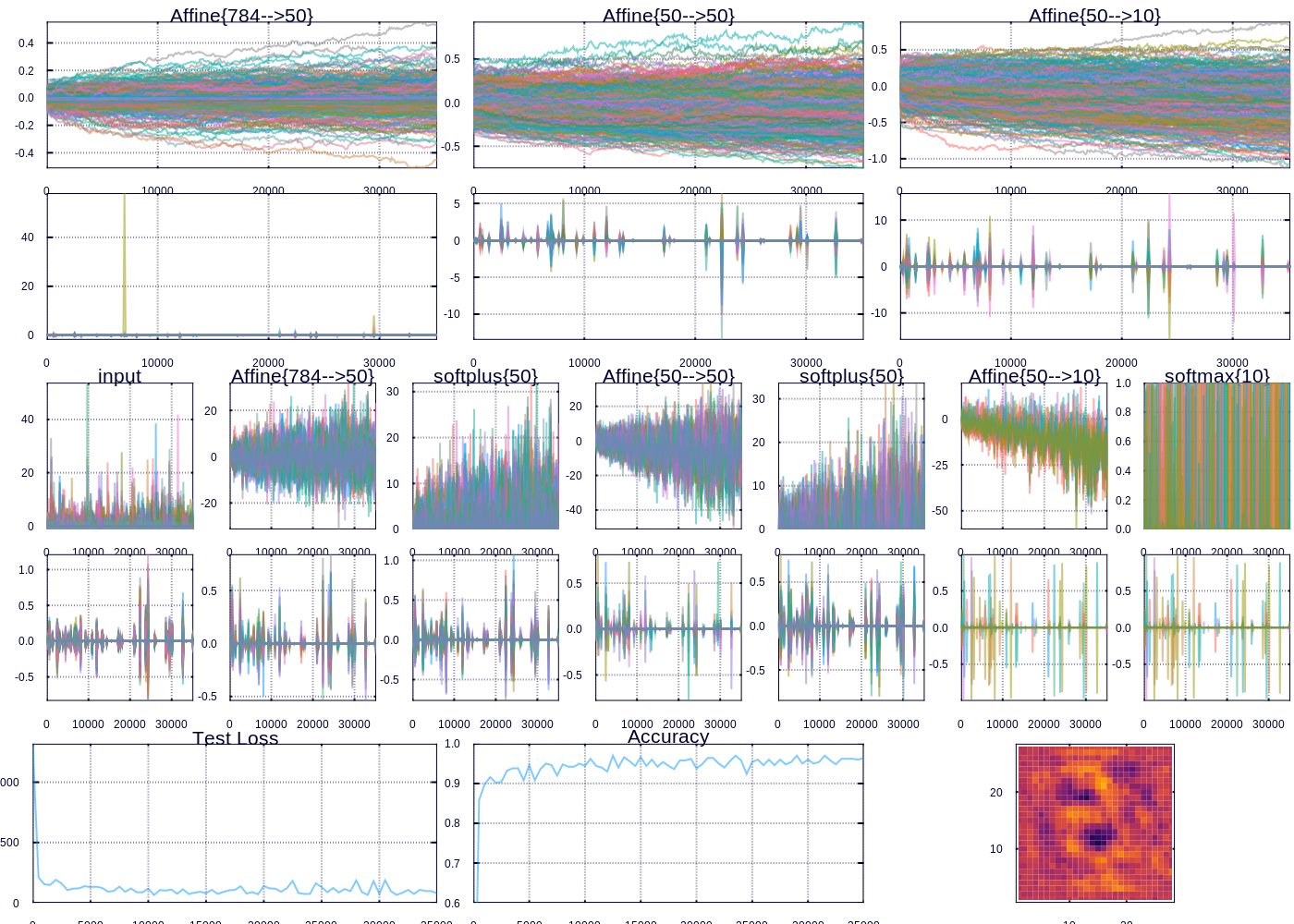
A snapshot after training for 30000 iterations
After a little while we are able to predict ~97% of the test examples correctly. The heatmap (which represents the “importance” of each pixel according to the outgoing weights of our model) depicts the important curves we have learned to distinguish the digits. The performance can be improved, and I might devote future posts to the many ways we could improve our model, however model performance was not my focus here. Rather I wanted to highlight and display the flexibility in learning and visualizing machine learning models.
Conclusion
There are many approaches and toolsets for data science. In the future, I hope that the ease of development in Julia convinces people to move their considerable resources away from inefficient languages and towards Julia. I’d like to see Learn.jl become the generic interface for all things learning, similar to how Plots is slowly becoming the center of visualization in Julia.
If you have questions, or want to help out, come chat. For those in the reinforcement learning community, I’ll probably focus my next post on Reinforce, AtariAlgos, and OpenAIGym. I’m open to many types of collaboration. In addition, I can consult and/or advise on many topics in finance and data science. If you think I can help you, or you can help me, please don’t hesitate to get in touch.